9 Lambda: First-class Functions🔗

9.1 First-class Functions🔗

Let us start turning the previous language, Fraud, into a real programming language. Let us say you write an expression to compute a particular value. Such an expression will only work for the single computation you have written down. For example, if you want to compute a factorial of 5, you will have to write a program (* 5 (* 4 (* 3 (* 2 1)))) that will compute the result as 120. If you want to find the factorial of any number, you will have to write down infinite number of expressions in Fraud. This means the expressiveness of our language is still severely restricted.

The solution is to bring in the computational analog of inductive data. Just like we can describe our programs by inductively composing each form in our language grammar, our language needs to be able to define arbitrarily long running computations. Crucially, these arbitrarily long running computations need to be described by finite sized programs. The analog of inductive data are recursive functions.

However, we will go one step further that just defining and using functions. We will also return functions and pass functions as arguments to programs, i.e., treat functions as values. Programming with functions as values is a powerful idiom that is at the heart of both functional programming and object-oriented programming, which both center around the idea that computation itself can be packaged up in a suspended form as a value and later run.

These functions in their most general form are called λ-expressions. We will add this to our language and call it Lambda.

9.2 Syntax🔗

First, we will look at how λs work in language in isolation and then add it to our main language. Here is the syntax for λ-expression:

(λ (x) e)

Here x is the formal parameter of the function and e is the body. Certain things are notable about this function expression:

• There is no function name in the λ-expression; it is an anonymous function.

• This new form is an expression — it can appear any where as a subexpression in a program.

Since functions are also considered values, functions can also be returned from a function. Thus, we can generalize what’s allowed in the function position of the syntax for function applications to be an arbitrary expression. That expression is expected to produce a function value (and this expectation gives rise to a new kind of run-time error when violated: applying a non-function to arguments), which can called with the value of the arguments. Hence the syntax of function applications is:

(e e)

In particular, the function expression can be a λ-expression, e.g.:

Racket REPL

> ((λ (x) (+ x x)) 10)

20

But also it may be expression which produces a function, but isn’t itself a λ-expression:

Racket REPL

> (let ((adder (λ (n) (λ (x) (+ x n)))))     ((adder 5) 10))

15

Here, (adder 5) is the function position of ((adder 5) 10). That subexpression is itself a function call expression, calling adder with the argument 5. It’s result is a function that, when applied, adds 5 to its argument. The argument on which the function is applied is called an actual parameter to the function. In this case 5 and 10 are the actual parameters.

While these are the key ideas, we will look at lambda expressions in a tiny language:

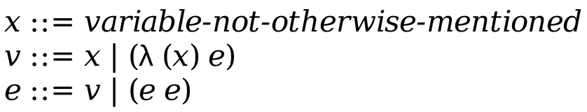
This above language is the Lambda Calculus. The lambda calculus was introduced in the 1930s by the logician Alonzo Church at Princeton University as a mathematical system for defining computable functions. Alan Turing (who was Church’s Ph.D. student) showed that the lambda calculus is equivalent in definitional power to Turing machines. The lambda calculus serves as the model of computation for functional programming languages and has applications to artificial intelligence, proof systems, and logic.

The programming language Lisp was developed by John McCarthy at MIT in 1958 around the lambda calculus. Haskell, considered by many as one of the purest functional programming languages, was developed by Simon Peyton Jones, Paul Houdak, Phil Wadler and others in the late 1980s and early 90s. Many established languages such as C++ and Java and many more recent languages such as Python, Ruby, and JavaScript have adopted lambda expressions as anonymous functions from the lambda calculus.

Because of its simplicity, lambda calculus is a very useful tool for the study and analysis of programming languages. It only has variables x, function abstractions (λ (x) e), written as (λx.e) as a short-hand, and function applications (e e). This is a tiny subset of the language we will design, but this is all we need to define all computable functions!

A function abstraction is a lambda expression that defines a function. It consists of four parts: a lambda followed by a variable, a period, and then an expression as in λx.e. Here, the variable x is the formal parameter of the function and e is the body of the function. For example, the function abstraction λx.x + 1 defines a function of x that adds x to 1. We say that λx.e binds the variable x in e and that e is the scope of the variable. Parentheses can be added to lambda expressions for clarity. Thus, we could have written this function abstraction as λx.(x + 1).

Note, we have minimized the syntax from the one used in Racket. This example does not illustrate the pure lambda calculus, because it uses the + operator, which is not part of the pure lambda calculus; however, this example is easier to understand than a pure lambda calculus example.

A function application, often called a lambda application, consists of an expression followed by an expression: e e. The first expression is a function abstraction and the second expression is the argument to which the function is applied. All functions in lambda calculus have exactly one argument. For example, the lambda expression λx.x + 1 2 or written more clearly as λx.(x + 1) 2 is an application of the function λx. (x + 1) to the argument 2.

Function application associates left-to-right; thus, f g h = (f g) h and it also binds more tightly than λ; thus, λx. f g x = (λx. (f g)x).

Functions in the lambda calculus are first-class citizens; that is to say, functions can be used as arguments to functions and functions can return functions as results.

9.3 Currying / Multi-argument functions🔗

All functions in lambda calculus are prefix and take exactly one argument. So how do we represent functions that take multiple arguments?

If we want to apply a function to more than one argument, we can use a technique called currying that treats a function applied to more than one argument to a sequence of applications of one-argument functions.

For example, to express the sum of two numbers x and y we can write λx.λy.x + y. To use this functions we have to apply it to two arguments in sequence. For example, to add 1 and 2, we use ((λx.λy.x + y) 1) 2. This is equivalent to a function in a programming language that allows multiple arguments. For example, in Racket and (our Lambda language syntax) the curried version looks like (((λ (x) (λ (y) (+ x y))) 1) 2), which is equivalent to ((λ (x y) (+ x y)) 1 2).

9.4 Free and Bound Variables🔗

In the function definition λx.x the variable x in the body of the definition (the second x) is bound because its first occurrence in the definition is λx. A variable that is not bound in expression e is said to be free in e. For example, in the function (λx.xy), the variable x in the body of the function is bound and the variable y is free.

Every variable in a lambda expression is either bound or free. Bound and free variables have quite a different status in functions.

• In the expression (λx.x)(λy.yx):

  • The variable x in the body of the leftmost expression is bound to the first lambda.

  • The variable y in the body of the second expression is bound to the second lambda.

  • The variable x in the body of the second expression is free.

  • Note that x in second expression is independent of the x in the first expression.

• In the expression (λx.xy)(λy.y):

  • The variable y in the body of the leftmost expression is free.

  • The variable y in the body of the second expression is bound to the second lambda.

We could check which variables are free using a free? function that accepts a list of bound variables, the variable we want to check is free, and an expression to check:

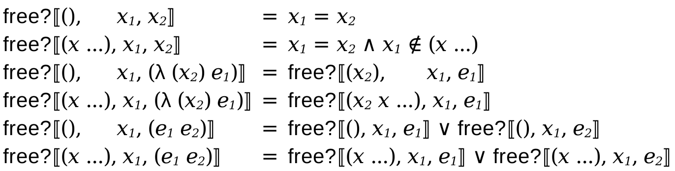
If the set of the bound variables is empty, a variable x1 is only free if the expression is only x1. Otherwise the variable x1 is free if it is not contained in the set of bound variables and the expression is x1. If the set of bound variables of empty, a variable x1 is free in λx2.e1 if x1 is free in e1 considering x2 as bound. Inductively, if the bound set is non-empty, the result is computed by including x2 in the set of bound variables. For function applications, x1 is free if it is free in either the function position e1 or free in the argument position e2.

9.5 Alpha Reductions🔗

A variable may occur more than once in some lambda expression; some occurrences may be free and some may be bound, so the variable itself is both free and bound in the expression, but each individual occurrence is either free or bound (but not both). For example, the free variables of the following lambda expression are {y,x} and the bound variables are {y}:

We need to distinguish between which y is free and the one that is bound. Given a lambda expression (λx.e1) e2 instead of replacing all occurrences of x in e1 with e2, we replace all occurrences of x that are free in e1 with e2. For example:

The issue here is that a variable x that is free in the original argument to a lambda expression becomes bound after rewriting (using that argument to replace all instances of the formal parameter), because it is put into the scope of a lambda with a formal that happens also to be named x:

To solve this, we use a technique called alpha reduction. The key idea is that formal parameter names are unimportant; so rename them as needed to avoid capture. Alpha reduction is used to modify expressions of the form λx.e. It renames all the occurrences of x that are free in e to some other variable z that does not occur in e (and then λx is changed to λz). For example, consider λx.λy.x + y (this is of the form λx.e). Variable z is not in e, so we can rename x to z; i.e., λx.λy.x + y alpha-reduces to λz.λy.z + y.

Here is alpha reduction formally defined as the α function. It takes the expression to be renamed, the variable to be renamed, and the new name of the variable. Crucially, the new name should be a fresh name, i.e., something that has not been used before.

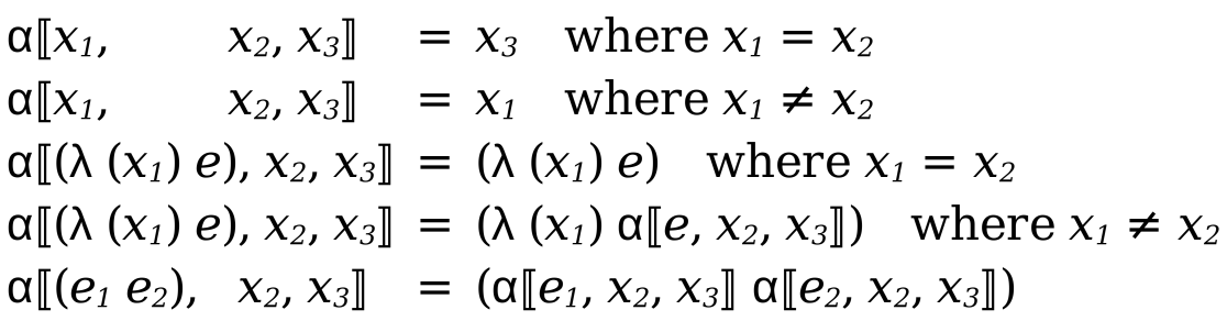
α renames a variable x1 to x3 only if x1 is the same variable as the one to be renamed x2. If the expression is a λ where the binding argument is same variable being replaced, there is nothing to substituted. Otherwise, the body of the λ is alpha renamed recursively. Function applications recursively call alpha reductions both in the function position and the argument position.

9.6 Beta Reductions🔗

A function application λx.e y is evaluated by substituting the argument y for all free occurrences of the formal parameter x in the body e of the function definition λx.e. This substitution is similar to the one presented in Fraud: Let Bindings and Variables. For example:

• (λx.x) y substitutes x = y in the body x and reduces to y.

• (λx.x z x) y substitutes x = y in the body x z x and reduces to y z y.

• (λx.z) y substitutes x = y in the body z and reduces to z since the formal parameter x does not appear in the body z.

This substitution in a function application is called a beta reduction. If we use substitution to transform e1 to e2, we say e1 reduces to e2 in one step. In general, (λx.e) y means that applying the function (λx.e) to the argument expression y reduces by substituting x with y in e, i.e., the argument expression y is substituted for the function’s formal parameter x in the function body e.

A lambda calculus expression (aka a "program") is "run" by computing a final result by repeatedly applying beta reductions, until we cannot reduce it any further. It is the reflexive and transitive closure of the term under substitution, i.e., zero or more applications of beta reductions. For example:

• (λx.x) y reduces to y (illustrating that λx.x is the identity function).

• (λx.x x) (λy.y) reduces to (λy.y) (λy.y) reduces to (λy.y); thus, we can say (λx.x x) (λy.y) evaluates to (λy.y). Note that here we have applied a function to a function as an argument and the result is a function.

Below is the behavior of beta reduction defined formally as the β function. The first argument is a term in which variables will be substituted. The second argument is the variable whose occurrence will be substituted. Finally, the third argument is the term that will be substituted in places of the second argument.

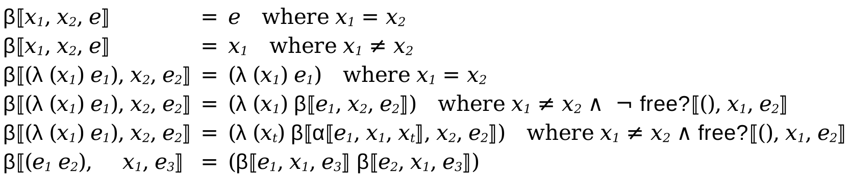
β substitutes a variable with e only if it is the same variable as the one to be substituted. If the expression is a lambda term and the variable to be substituted if rebound in the lambda term, it is returned as-is. Otherwise, if the rebound variable in the lambda is not free, the body of the lambda can be beta reduced recursively. However, if the rebound variable in the lambda is free, then we need a fresh variable name xt, and alpha rename the lambda body followed by beta reduction of the lambda body. Finally, for function application, beta reduction is recursively doing beta reduction on the function position term and the argument position term.

9.7 Meaning of a Lambda Expression🔗

A lambda calculus expression can be thought of as a program which can be executed by evaluating it. Evaluation is done by repeatedly finding a reducible expression (called a redex) and reducing it by a function evaluation until there are no more redexes.

Example 1: The lambda expression (λx.x) y in its entirety is a redex that reduces to y.

Example 2: The lambda expression (+ (* 1 2) (− 4 3)) has two redexes: (* 1 2) and (− 4 3). If we choose to reduce the first redex, we get (+ 2 (− 4 3)). We can then reduce (+ 2 (− 4 3)) to get (+ 2 1). Finally we can reduce (+ 2 1) to get 3.

The term beta reduction is perhaps misleading, since doing beta reduction does not always produce a smaller lambda expression. In fact, a beta reduction can:

• decrease,

• increase,

• not change

the length of a lambda expression. Below are some examples. In the first example, the result of the beta-reduction is the same as the input (so the size doesn’t change); in the second example, the lambda expression gets longer and longer; and in the third example, the result first gets longer, and then gets shorter.

• (λx.xx)(λx.xx) reduces to (λx.xx)(λx.xx)

• (λx.xxx)(λx.xxx) reduces to (λx.xxx)(λx.xxx)(λx.xxx) reduces to (λx.xxx)(λx.xxx)(λx.xxx)(λx.xxx)

• (λx.xx)(λa.λb.bbb) reduces to (λa.λb.bbb)(λa.λb.bbb) reduces to λb.bbb

9.8 Reduction Strategy🔗

A program can be reduced to find the resulting value. In other words, it takes a reducible expression, or redex, and reduces it using the reduction rules. However, here also multiple choices are available when reducing a term and a reduction strategy specifies the order in which beta reductions are made.

Some reduction orders for a lambda expression may yield a normal form while other orders may not. For example, consider the expression: (λx.z)((λx.x x)(λx.x x))

This expression has two redexes:

• The entire expression is a redex in which we can apply the function (λx.z) to the argument ((λx.x x)(λx.x x)) to yield the normal form z. This redex is the leftmost outermost redex in the given expression.

• The subexpression ((λx.x x)(λx.x x)) is also a redex in which we can apply the function (λx.x x) to the argument (λx.x x). Note that this redex is the leftmost innermost redex in the given expression. But if we evaluate this redex we get same subexpression: (λx.x x)(λx.x x) → (λx.x x)(λx.x x). Thus, continuing to evaluate the leftmost innermost redex will not terminate and no normal form will result.

As a second example, consider the expression: (λx. λy. y)((λz.z z)(λz.z z))

This expression has two redexes:

• The entire expression is a redex in which we apply the function (λx. λy. y) to the argument ((λz.z z)(λz.z z)) to yield the normal form (λy. y). This redex is the leftmost outermost redex in the given expression.

• The subexpression ((λz.z z)(λz.z z)) is also a redex in which we can apply the function (λz.z z) to the argument (λz.z z). Note that this redex is the leftmost innermost redex in the given expression. But if we evaluate this redex we get same subexpression: ((λz.z z)(λz.z z)) → ((λz.z z)(λz.z z)). Thus, continuing to evaluate the leftmost innermost redex will not terminate and no normal form will result.

In general, there are two orders for evaluating lambda expressions:

• Normal Order: Replace bound variables by unevaluated argument expressions. The leftmost outermost redex is always reduced first and the arguments are substituted into the body before reduction. Often this is known as call-by-name.

  

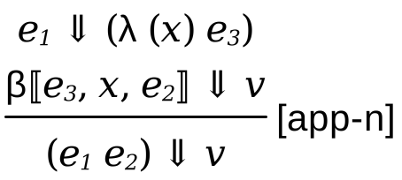
  Thus to give meaning to function application using call-by-name reduction semantics, we have to find the meaning of the function position term e1 which should be a lambda. Then argument position term e2 is substituted in the body of the lambda e3 in the place of x using beta reduction which gives us the meaning of the entire function application.

• Applicative order: Broadly, replace the bound variables with the value of the argument expression. The leftmost innermost redex is always reduced first. Intuitively this means a function’s arguments are always reduced before the function itself. Often this is known as call-by-value.

  

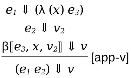
  Thus to give meaning to function application using call-by-value reduction semantics, we have to find the meaning of the function position term e1 which should be a lambda and the meaning of the argument e2 as v2. Then v2 is substituted in the body of the lambda e3 in the place of x using beta reduction which gives us the meaning of the entire function application.

For pure programs, i.e., programs without side effects, the call-by-name reduction strategy is a superset of call-by-value. If there exists a reduction to a value, call-by-name will find it, but the same may not hold true for call-by-value. Inversely, if call-by-value reduces a term to a value, a call-by-name evaluation will evaluate it to a value as well. If they run to completion, they will always reduce the same expression to the same value.

9.9 Interpreter for Lambda Calculus🔗

To define the interpreter for the lambda calculus, we first need to translate the definitions of free?, α, and β to code. All individual cases in in those above definitions become pattern matches and when we need the fresh variable name in the beta reduction we use the Racket builtin function gensym to get us a fresh symbol name each time:

lambda/interp.rkt

#lang racket

(provide free? alpha-reduce beta-reduce)

; Listof Var -> Var -> Expr -> Bool

(define (free? xs x e)

(match e

[(? symbol?)  (and (eq? e x) (not (memq x xs)))]

[`(λ (,y) ,e) (free? (cons y xs) x e)]

[`(,e1 ,e2)   (or (free? xs x e1) (free? xs x e2))]))

; Expr -> Var -> Var -> Expr

; z has to be fresh

(define (alpha-reduce e x z)

(match e

[(? symbol?)  (if (eq? x e) z e)]

[`(λ (,y) ,e) (if (eq? x y)

`(λ (,x) ,e)

`(λ (,y) ,(alpha-reduce e x z)))]

[`(,e1 ,e2)   `(,(alpha-reduce e1 x z) ,(alpha-reduce e2 x z))]))

; Expr -> Var -> Expr -> Expr

(define (beta-reduce e1 x e2)

(match e1

[(? symbol?)  (if (eq? e1 x) e2 e1)]

[`(λ (,y) ,e) (if (eq? x y)

`(λ (,y) ,e)

(if (not (free? '() y e2))

`(λ (,y) ,(beta-reduce e x e2))

(let* ((ry (gensym))

(re (alpha-reduce e y ry)))

`(λ (,ry) ,(beta-reduce re x e2)))))]

[`(,ea1 ,ea2) `(,(beta-reduce ea1 x e2) ,(beta-reduce ea2 x e2))]))

We can run these functions to see if they behave as expected:

Now, all we have to do is decide a reduction strategy and build an interpreter.

9.9.1 Call-by-name🔗

A call-by-name interpreter only reduces the function position term before beta-reduction and then interprets the reduced term again.

Let us see an example of two terms that evaluates to a value using call-by-name:

9.9.2 Call-by-value🔗

A call-by-name interpreter reduces both the function position term and the argument position term before beta-reduction and then interprets the reduced term again.

Let us try to run the same two terms using call-by-value again:

Notice how the second example reduces successfully using call-by-name but gets stuck using call-by-value reduction?

9.9.3 Intermediate Steps🔗

To see how call-by-name differs from call-by-value, we can look at the intermediate steps of the reduction. For that all we have to do is remove the recursive call to the interpreter around our beta reduction.

For call-by-name, it looks like:

Notice how we added a case for *? It allows us to write more interesting programs that do arithmetic:

Thus, the expression (* 2 3) is substituted directly. We can continue running until we get the value:

Let us contrast this to a call-by-value interpreter that shows the intermediate steps:

Let us run the same expression again:

Thus, the expression (* 2 3) is evaluated and then substituted. We can continue running until we get the value:

9.10 Adding Lambdas to our Language🔗

We can now take these core ideas and implement this in our existing interpreter. Below is an implementation that shows how it looks when our language has integers, arithmetic operations like * and -, if, and let. You can try extending these definitions for the rest of the language on your own. We are using call-by-name semantics below, but you can changing the reduction semantics on your own to see how the behavior changes.

lambda/interp-full.rkt

#lang racket

(provide free? alpha-reduce beta-reduce interp)

; Listof Var -> Var -> Expr -> Bool

(define (free? xs x e)

(match e

[(? integer?) #f]

[(? symbol?)  (and (eq? e x) (not (memq x xs)))]

[`(λ (,y) ,e) (free? (cons y xs) x e)]

[`(zero? ,e) (free? xs x e)]

[`(- ,e1 ,e2) (or (free? xs x e1) (free? xs x e2))]

[`(* ,e1 ,e2) (or (free? xs x e1) (free? xs x e2))]

[`(if ,e1 ,e2 ,e3) (or (free? xs x e1) (free? xs x e2) (free? xs x e3))]

[`(let ((,y ,e1)) ,e2) (or (free? xs x e1) (free? (cons y xs) x e2))]

[`(,e1 ,e2)   (or (free? xs x e1) (free? xs x e2))]))

; Expr -> Var -> Var -> Expr

; z has to be fresh

(define (alpha-reduce e x z)

(match e

[(? integer?) e]

[(? symbol?)  (if (eq? x e) z e)]

[`(λ (,y) ,e) (if (eq? x y)

`(λ (,x) ,e)

`(λ (,y) ,(alpha-reduce e x z)))]

[`(zero? ,e) `(zero? ,(alpha-reduce e x z))]

[`(- ,e1 ,e2) `(- ,(alpha-reduce e1 x z) ,(alpha-reduce e2 x z))]

[`(* ,e1 ,e2) `(* ,(alpha-reduce e1 x z) ,(alpha-reduce e2 x z))]

[`(if ,e1 ,e2 ,e3) `(if ,(alpha-reduce e1 x z) ,(alpha-reduce e2 x z) ,(alpha-reduce e3 x z))]

[`(let ((,y ,e1)) ,e2) (if (eq? x y)

`(let ((,x ,(alpha-reduce e1 x z))) ,e2)

`(let ((,y ,(alpha-reduce e1 x z))) ,(alpha-reduce e2 x z)))]

[`(,e1 ,e2)   `(,(alpha-reduce e1 x z) ,(alpha-reduce e2 x z))]))

; Expr -> Var -> Expr -> Expr

(define (beta-reduce e1 x e2)

(match e1

[(? integer?) e1]

[(? symbol?)  (if (eq? e1 x) e2 e1)]

[`(λ (,y) ,e) (if (eq? x y)

`(λ (,y) ,e)

(if (not (free? '() y e2))

`(λ (,y) ,(beta-reduce e x e2))

(let* ((ry (gensym))

(re (alpha-reduce e y ry)))

`(λ (,ry) ,(beta-reduce re x e2)))))]

[`(zero? ,e) `(zero? ,(beta-reduce e x e2))]

[`(- ,ea1 ,ea2) `(- ,(beta-reduce ea1 x e2) ,(beta-reduce ea2 x e2))]

[`(* ,ea1 ,ea2) `(* ,(beta-reduce ea1 x e2) ,(beta-reduce ea2 x e2))]

[`(if ,ea1 ,ea2 ,ea3) `(if ,(beta-reduce ea1 x e2) ,(beta-reduce ea2 x e2) ,(beta-reduce ea3 x e2))]

[`(let ((,y ,ea1)) ,ea2) (if (eq? x y)

`(let ((,x ,(beta-reduce ea1 x e2))) ,ea2)

`(let ((,y ,(beta-reduce ea1 x e2))) ,(beta-reduce ea2 x e2)))]

[`(,ea1 ,ea2) `(,(beta-reduce ea1 x e2) ,(beta-reduce ea2 x e2))]))

; Expr -> Val

(define (interp e)

(match e

[`(zero? ,e)             (eq? (interp e) 0)]

[`(- ,ea1 ,ea2)          (- (interp ea1) (interp ea2))]

[`(* ,ea1 ,ea2)          (* (interp ea1) (interp ea2))]

[`(if ,ea1 ,ea2 ,ea3)    (match (interp ea1)

[#f (interp ea3)]

[_  (interp ea2)])]

[`(let ((,x ,ea1)) ,ea2) (interp (beta-reduce ea2 x ea1))]

[`(,e1 ,e2)              (match (interp e1)

[`(λ (,x) ,e) (interp (beta-reduce e x e2))]

[(? symbol? x) x])]

[_                       e]))

Most operations push free?, alpha-reduce, beta-reduce, and interp to the inner terms. The only exception is let: we have to be careful to handle the changes it makes to the variable bindings.

Let us use this interpreter to encode different language features just using lambdas to show you that lambdas are all you need!

9.11 Encoding programs in Lambda Calculus🔗

So far we look at how we can compute with lambda expressions. Turns out we can encode any behavior of a computable program in a lambda expression. This means we can encode all language features we developed until now (or any feature you want from your favorite language) as lambda expressions!

9.11.1 Let Bindings🔗

Let us recall what a let binding like (let ((x e1)) e2) did: it bound e1 to x, and made x a bound variable in the expression e2. This is infact what lambdas do as well.

A lambda term ((λx.e2) e1) is exactly the same — it evaluates to e2, while binding x to e1. We can actually run this through our interpreter to confirm it is correct:

9.11.2 Conditionals and Boolean Values🔗

First, let’s consider how to encode a conditional expression: (if p a b) (i.e., the value of the whole expression is either a or b, depending on the value of p). We will represent this conditional expression using a lambda expression of the form: (cond p a b), where cond, p, a and b are all lambda expressions. In particular, cond is a function of 3 arguments that works by applying p to a and b (i.e., p is the condition and a is the then-branch and b is the else branch):

cond ::= λp.λa.λb.p a b

To make this definition work correctly, we must define the representations of true and false carefully (since the lambda expression p that cond applies to its arguments a and b will reduce to either true or false). In particular, when true is applied to a and b we want it to return a, and when false is applied to a and b we want it to return b. Therefore, we will let true be a function of two arguments that ignores the second argument and returns the first argument, and we’ll let false be a function of two arguments that ignores the first argument and returns the second argument:

true ::= λx.λy.x

false ::= λx.λy.y

Now let’s consider an example: cond true m n. Note that this expression should evaluate to m. Let’s see if it does (by substituting our definitions for cond and true, and evaluating the resulting expression). The sequence of beta reductions is shown below; in each case, the redex about to be reduced is indicated by underlining the formal parameter and the argument that will be substituted in for that parameter.

We can run such programs through Racket and confirm our understanding is correct:

We can go and replace all the let-s to encode this purely using lambdas. It is not very readable, but it is the same program:

9.12 Y-Combinator🔗

We have one final issue to deal with: recursive functions. For example, consider how we can write the factorial function in Racket:

This crucially relies on the ability to name our functions. Without the ability to call the function fact, how do we recursively call it? If adding lambdas to our language makes it truly a general computing language we should be able to do recursion.

To do this we use the Y-combinator in lambda calculus which is defined as:

λf.(λy.f(y y))(λy.f(y y))

This computes the fix-point of a function in call-by-name reduction semantics, i.e., the result of applying the function repeatedly until it terminates. Assuming you are applying the the Y-combinator to a function g:

Thus the Y-combinator continues running g until g reaches a fix-point, i.e., terminates.

Let us write the factorial function using the Y-combinator:

The definition of fact changes to accept a lambda that is called recursively from the function body. Calling (fact 5) produces the factorial of 5, 120.

We could get rid of the let-s and use pure lambdas:

9.13 Discussion🔗

We should take a pause, and appreciate the milestone we have reached. Our Lambda language implements an elaborate version of the Lambda Calculus—a general purpose programming language. Thus, the language Lambda can represent all possible computation one can ever represent in any general purpose language (including C, C++, Java, Ruby, Python, JavaScript, Haskell).

If our language can express all kinds of programs, we are done, right? What should we do for the latter half of the semester? Think on it!